0:05
How exactly does a physical change
0:07
inside a pipe, like fluid pressure, turn
0:10
into a precise electrical signal that a
0:12
computer can read? To understand the
0:14
process, we'll use a standard example. A
0:17
pressure transmitter calibrated to a
0:19
range of 0 to 10 bar.
0:21
Our first step is to define the total
0:23
physical window of that instrument by
0:25
calculating the span. By subtracting the
0:28
lower range value from the upper range
0:30
value, we find a span of 10 bar.
0:33
Defining the span establishes the
0:35
mathematical boundaries for the entire
0:37
loop. Without this physical context, the
0:40
electrical current being sent to the
0:41
controller has no specific meaning. If
0:44
the physical process variable, or PV, is
0:47
currently reading 7.5 bar, we first need
0:50
to determine where that value sits
0:51
proportionally within our 10 bar span.
0:54
Subtracting the lower range value before
0:57
dividing by the span is a critical step.
0:59
While it seems simple when the LRV is
1:02
zero, building this habit ensures
1:04
accuracy when working with instruments
1:06
that have an offset, like a vacuum
1:08
gauge. Here, the calculation puts us at
1:11
75% of the span. Now, we map that 75%
1:15
onto the electrical scale using the
1:17
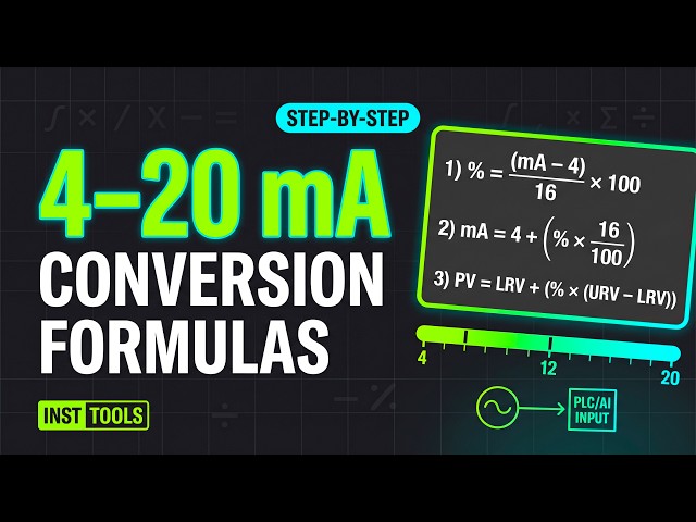
formula for loop current. We multiply
1:20
the percentage by 16 because the total
1:22
electrical span is 16 milliamps, the
1:25
difference between 4 and 20. We then add
1:28
the 4 milliamp baseline. This live zero
1:31
ensures the system can tell the
1:32
difference between a zero pressure
1:34
reading and a snapped wire.
1:36
Normalizing physical measurements into a
1:38
percentage first allows this same
1:40
conversion logic to be applied to any
1:42
instrument in the plant, regardless of
1:45
whether it measures pressure,
1:46
temperature, or flow. If we look at the
1:48
signal from the PLC's perspective, we
1:50
might see an incoming signal of 12
1:52
milliamps. To find the physical
1:54
pressure, we have to reverse the math.
1:56
Order of operations is key here.
1:59
You must strip away the 4 milliamp
2:01
baseline before dividing by the 16
2:04
milliamp current span. This tells us the
2:06
signal is at exactly 50% of the
2:09
transmitter's range. You can also use a
2:11
combined formula to translate the
2:13
current directly back into physical
2:15
pressure without calculating the
2:16
percentage as a separate step. By
2:19
scaling the percentage against the
2:20
physical span and adding the LRV back
2:23
in, the formula converts 12 milliamps
2:25
back into the 5 bar reading.
2:28
Try to combine these steps yourself.
2:30
Without stopping to find the percentage
2:32
first, write a single formula to
2:34
calculate the milliamp signal for a PV
2:38
Mastering these calculations allows you
2:40
to cross reference a field gauge with a
2:44
If your calculated value doesn't match
2:45
the screen, you've effectively narrowed
2:47
the problem down to either a scaling
2:49
error in the PLC or a calibration drift
2:52
in the transmitter. This direct formula
2:54
combines previous steps into one line.
2:57
It takes the physical reading, finds the
2:59
percentage, and applies the milliamp
3:01
scale. Running our 7.5 bar PV confirms
3:05
the 16 milliamp result. These three
3:08
quick checks verify loop function
3:11
You may want to screenshot this summary
3:13
grid. It organizes the formulas by their
3:15
end goal, providing a quick reference
3:17
for calculating span, percentages, and
3:21
These formulas ensure that every step of
3:23
the conversion process is verifiable.
3:26
Applying them correctly maintains a
3:27
predictable mathematical link between
3:29
the physical process and the control