Up next in 10

RDD Operation Transformations
Show More Show Less View Video Transcript
0:00
in this video we are discussing RDD
0:03
operations and you are discussing
0:05
transformations we knew that on a DD 2
0:08
kind of operations can be carried out
0:09
one is the transformations another one
0:12
is the actions in case of our DD
0:14
transformation it will take one or DD as
0:17
input and it can produce multiple rdd's
0:20
as output in this session you are
0:22
discussing only the transformations
0:24
operations so let us go into further
0:27
details so inspark
0:31
are DD there are two type of operations
0:33
of the earth one is the transformations
0:35
another one is the actions in case of
0:38
transformations the Arditi
0:39
transformations are some functions that
0:41
take one or DD as input and from one or
0:45
more than our duties will be obtained as
0:48
output so one or DD will be taken as
0:51
input and one or more our duties will be
0:53
obtained as the output
0:55
we know that our distance for resilient
0:57
distributed data set and this is nothing
1:01
but one data structure with the help of
1:03
which a data set can be distributed into
1:06
multiple servers multiple nodes so that
1:08
multiple processors can work on them
1:10
simultaneously at the same time all our
1:13
T DS are immutable
1:15
then the main our DD will not be changed
1:18
the these are duties are immutable here
1:21
so as a result of that this Manor DD
1:23
cannot be changed it is lazy operation
1:27
though it creates some art it is but
1:29
they execute when an action is called so
1:33
it is a lazy computing that means
1:34
whenever one action will be called then
1:37
this competition will take place to
1:41
improve the competition performance we
1:43
can set some transformations as
1:45
pipelined so we can have some
1:48
transformations to be carried out
1:49
pipeline that means one operations
1:51
output will be the next operations input
1:54
so in this way we can create one
1:55
pipeline and it will it will get
1:57
completed when the pipeline all the
1:59
operations mentioned in the pipeline
2:01
will get completed so it helps to
2:04
optimize the process so there are two
2:06
kinds of transformations one is the
2:08
narrow transformation another one is the
2:11
wide transformation in case of narrow
2:13
transformation we know that it will take
2:16
a partition as input and it will produce
2:18
the respective outputs in under the
2:20
partition that means it is not involving
2:23
all the partitions in case of nano
2:25
transformation but in case of Y
2:27
transformation it is doing the
2:29
operations on multiple partitions taking
2:32
them as input so let us go for some
2:35
further discussion on it so at first we
2:37
are concentrating on narrow
2:39
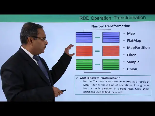
transformation you can find that we are
2:41
here you are having multiple different
2:43
partitions are there and respective
2:45
partitions will be obtained as output if
2:47
we carry out some operations like your
2:50
map flatmap map partition filter sample
2:54
union so these are the different
2:56
operations are there so what is narrow
2:59
transformation narrow transformations
3:01
are generated as a result of map filter
3:04
or other kind of operations as we have
3:07
mentioned there and it originates from a
3:10
single partition in the parent RDD that
3:13
means it is not involving multiple
3:15
partitions of the parent RDD and only
3:18
some partitions used to find the
3:20
respective result so that's why it is
3:22
called the Nano partition because all
3:25
partition partitions are not having that
3:27
participation in these operations now
3:31
let us go for wide transformation and
3:34
here you can find that there here we are
3:37
having multiple partitions are there and
3:39
you can see that multiple partitions are
3:41
taking participation in the operation to
3:44
produce the output partitions and that's
3:46
why also it is known as shuffle
3:48
operation so you can find that here you
3:51
have made different colors for different
3:52
partitions you can see the the outcome
3:55
partitions are containing the respective
3:57
portions for multiple different input
3:59
partitions and the operations may be
4:01
intersection distinct reduced by key
4:04
group by key join Kardashian repartition
4:08
and qualies so why transformations are
4:12
generated as a result of group by key
4:15
reduced by key or these kind of
4:17
operations in this case to form a data
4:20
partition it can take data from more
4:22
than one partitions you can see that it
4:25
is taking data
4:26
more than one partitions and it is also
4:28
known as saffle partition so here we
4:31
have discussed that is our DT operation
4:33
that is transformations thanks for
4:36
watching this video
#Programming