0:00
In this video we are going to discuss distribution shapes
0:04
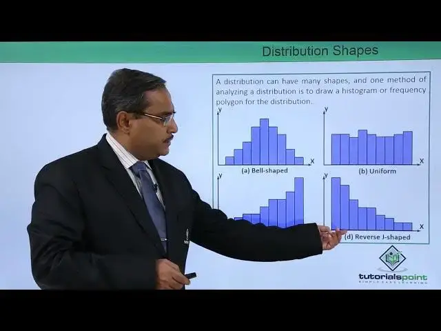
A distribution can have many shapes and one method of yzing a distribution is to draw a
0:13
histogram or frequency polygon for the distribution. In the earlier video we have discussed what is histogram, what are its disadvantages and advantages
0:24
what is frequency polygon and also a jeep. So here you can find that to be a histogram
0:29
to get the distribution shapes, we should draw the frequency polygon or the respective histograms
0:37
So, if the histogram is having a shape like this, so you can find that it is having a good tendency
0:44
towards the central. So, there is a central tendency is high for this particular data set
0:49
because the density in the center is very much high, and it is known as bell shaped. Otherwise
0:55
for this type of distribution shapes, we can call it as a..
0:58
uniform shape This is known as the J shaped if the distribution is something like this because we are getting the most of the data is falling in the higher value for X in the higher class intervals
1:13
And this is known as the reverse J shape. Here most of the frequencies, the most of the frequencies are falling in the lower class
1:19
limits, lower class intervals you can find. This is the right skewed
1:27
This is the right skewed. this sort of distribution shape will be called as right skewed
1:32
This is our left skewed. Here the frequency is less in the first few class intervals and then the frequency is growing
1:41
And this is known as bi-modal because there are two class intervals having got highest frequencies
1:47
So that is known as bi-modal and this sort of shape is known as U-shaped
1:52
So from this histograms we are getting the idea about the frequency distribution shapes
1:58
of our data. From where we can do multiple different conclusions we can reach and that's
2:05
why distribution shapes are very vital. Thanks for watching this video