Up next in 10

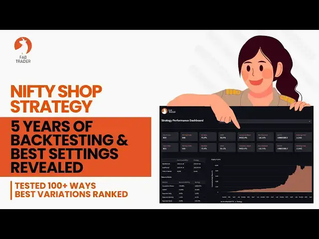
Nifty Shop Swing Strategy Backtested for 5 Years and Best Settings Revealed | Mahesh Chander Kaushik
Aug 12, 2025
Backtesting the Nifty SHOP Strategy over 5 years with 3 different position sizing methods — Static, Percentage of Cash, and the new Divisor Method. The best combination of inputs that provides the maximum results revealed!
In this deep dive, I:
✅ Test multiple target , averaging settings and position sizing approaches
✅ Compare risk, returns, and consistency
✅ Rank all combinations using my custom StratRanker Sheet
✅ Reveal the top-performing settings for long-term compounding
You’ll see exactly how the Divisor method works — a powerful compounding approach where position size grows as your portfolio grows.
📌 Resources mentioned in this video:
Download Python Backtest Script, Daily Screener, Tradebooks & Ranking Sheet:
https://fabtrader.in/product/nifty-shop-strategy-screener-and-core-logic/
Master Strategy Backtesting using Python and AI Course (No Coding Experience needed)
https://fabtrader.in/course/master-trading-strategy-backtesting-with-ai-and-python/
Build Your Own Algo Trading Platform – Step-by-step Python course - Flagship Course: https://fabtrader.in/course/build-your-own-algo-trading-system-in-python/
Show More Show Less View Video Transcript
0:01
Hello everyone. Uh over the last few
0:02
weeks, my inbox was uh flooded with
0:04
messages from our FAR trader community
0:06
members. Uh many of you saw my previous
0:08
video on the Nifty shop strategy where I
0:10
shared my live trades and returns and
0:13
the the feedback has been incredible,
0:14
right? So a lot of you were excited,
0:16
some of you were curious and quite a few
0:18
asked me the same question. Can this be
0:20
back tested? So in today's video, we're
0:23
going to do exactly that. uh we're going
0:25
to take the nifty shop strategy, put it
0:27
through five years of data, test
0:28
multiple variations of the rules,
0:30
multiple combinations of the input
0:31
consideration, measure its performance
0:33
not just on the returns but also on the
0:35
risk and consistency and finally I'll
0:37
share with you the top ranked
0:38
combinations that yielded the best
0:40
returns over the past 5 years. So stick
0:42
around till the end because I'm going to
0:43
reveal the winner the the best
0:45
combination that produced the the best
0:46
results and the returns for Nifty Shop
0:49
strategy. Now, for those of you who
0:51
might be new here and didn't watch the
0:53
first video, please watch that video
0:54
first to get a full understanding of
0:55
what the strategy is all about. I've
0:56
shared the link to this video in the
0:58
description. However, let me give you a
0:59
quick refresher on what this Nifty shop
1:01
strategy is all about. This strategy is
1:03
built on the promise that the Nifty50
1:05
stocks, the largest and the most stable
1:07
companies in India, rarely stay down for
1:09
too long, right? So, we look for
1:10
temporary pullbacks in these
1:11
fundamentally strong stocks. Enter when
1:13
they are significantly below their
1:14
20-day moving average and then patiently
1:16
wait for them to revert back up, right,
1:18
to a to a set target before selling,
1:20
right? There's no stop- loss in this
1:21
strategy. We average down when the price
1:23
drops further and uh sell when our
1:25
average cost hits the the target. So,
1:27
it's simple, mechanical, and ideal for,
1:29
you know, kind of beginners or busy
1:30
professionals who want steady
1:32
compounding without the stress of, you
1:33
know, watching the charts all day.
1:35
Again, I strongly urge that you watch
1:36
the other video first before you proceed
1:38
with this one. Now, let's talk about the
1:40
entry rules. Uh, you only need about 10
1:41
minutes a day uh at around 3:20 p.m. As
1:44
you know, 3:30 is when the market
1:45
closes. So, it's 10 minutes before the
1:47
market close. U step one, you just scan
1:49
for uh, you know, the the Nifty50
1:51
universe of stocks and find five stocks
1:53
that are trading the farthest below
1:54
their 20-day moving average. That's step
1:56
number one.
1:58
Step number two is from those five, pick
2:01
one stock that you already don't have,
2:03
right? That you already don't hold and
2:05
then buy it. If all the five stocks uh
2:07
you know that that was chosen for that
2:09
particular day are already part of your
2:10
portfolio then you look for averaging
2:12
down opportunity. In this strategy you
2:14
average down only when a stock from your
2:16
holding has fallen more than 3% from
2:18
your last buy price. And once you do
2:20
that you buy only one stock per day that
2:22
has fallen the most. And now for the
2:24
exit rules at the end of the day before
2:26
you actually begin the buy leg of the
2:27
strategy you do the following steps to
2:29
sell the stocks that are eligible.
2:30
Right? So at 3:20 uh p.m. every day, you
2:34
check your portfolio and see if any
2:35
stock that is trading more than 5% above
2:38
your average buy price, right? The 5% is
2:40
the target and uh that we've kept for
2:42
this particular strategy. And if you do
2:44
have any stock which satisfies that
2:46
condition, you just sell one stock per
2:48
day.
2:50
So this is the original strategy.
2:51
However, based on our back test results,
2:53
we're going to change a few things uh to
2:54
take it from from good to awesome
2:56
levels, right? So stay with me on that.
2:59
This is an interesting part. Uh we've
3:01
come to the position sizing approach
3:02
here. The original strategy if you
3:04
remember recommended a few approaches to
3:05
position sizing. However, I took a fresh
3:07
look at it and I have considered the
3:08
following three approaches for my back
3:09
testing. Number one is these static
3:12
position sizing. So in this we assume a
3:14
set amount for each trade and that
3:16
amount won't change. For example, 10,000
3:18
rupees for each trade when you buy a
3:19
stock for the first time and then the
3:21
same 10,000 when you are averaging down.
3:23
Right? Here I've also considered two
3:25
other variations within it which is one
3:27
is pyramiding where if you allocate
3:29
10,000 when you buy a stock for the
3:30
first time then you allocate a smaller
3:32
amount say 5,000 for averaging. The
3:34
reverse pyramid is also possible where
3:36
you use 10,000 for the first buy and
3:38
then you allocate 15,000 for averaging
3:40
right the advantage with this one is
3:42
that since you're since you're basically
3:43
averaging with a higher amount the
3:44
position can come up to target much
3:46
faster. So for the back testing we will
3:48
use all these variations and then you'll
3:50
see all our detail shortly. The second
3:52
approach is the dynamic approach where
3:54
we go for a percentage of the free cash
3:55
that is available. For example, let's
3:58
say you start with four lakhs and you
3:59
already have used three lakhs and have
4:01
only one lakh left within your
4:02
portfolio. Right? Then your position
4:04
size will be like 5% of that one lakh
4:06
which is 5,000 per trade. Right? Here as
4:09
well we will change the percentage point
4:11
increase it decrease it you know uh and
4:13
then test various different combinations
4:14
within our back testing. The third
4:16
approach is the divisor approach wherein
4:18
you divide the total portfolio value by
4:20
a number called the divisor. For
4:22
example, let's say 40 is your divisor
4:23
and your portfolio value is say four
4:25
lakhs. So four lakhs divided by 40 and
4:27
that will be 10,000 per trade will be
4:29
your position size. Here as well, we can
4:32
change the divisor number up and down to
4:33
see which divisor value gives us the
4:35
best results. So given all this
4:37
background, we have multiple inputs into
4:39
the strategy that needs to change and we
4:41
need to test all possible combinations
4:43
to see which one basically comes up at
4:44
the top. Right? So to recap, what are
4:47
the variables within the strategy? There
4:48
are four main variables or four levers
4:50
that we are going to be leveraging.
4:53
Number one, the the position size of the
4:56
first bite. The second is the position
4:57
size of the averaging. Right? The
4:59
thirdly, the target percentage. While
5:01
the original strategy told us to keep a
5:03
5% target, we're going to change this
5:05
number as well. And lastly, the fall
5:07
percentage of averaging down. The
5:09
original strategy told us that we only
5:11
consider for averaging down if the stock
5:13
in our holding has already fallen down
5:15
by 3%. So what if we vary this number 3%
5:18
to say 4 5 6%. And how would that impact
5:22
the overall performance of the strategy
5:23
and that's what we're going to be also
5:24
doing as part of our back testing. So as
5:27
you can see there are many permutations
5:29
and combinations that would basically
5:31
run into thousands of scenarios and it
5:33
is humanly not possible to test every
5:35
one of those. However, I've considered
5:37
around 40 such scenarios for my testing
5:39
and I've back tested each one of those.
5:41
This is all okay. But we have a new
5:43
challenge, right? We are testing so many
5:44
variations. How do we decide which one
5:46
is better? Right? And that's where I use
5:48
my simple framework that I learned from
5:50
a friend of mine who who runs a PMS,
5:52
right? While there are hundreds of
5:53
strategy performance metrics, it is
5:55
impossible to compare all those numbers.
5:57
Right? So, I personally broadly look at
5:59
three aspects. Number one is the
6:00
returns, risk, and probability. Where
6:03
all these three kind of come together.
6:04
Uh that's the sweet spot in the middle
6:06
that we are basically going to look for
6:08
and measure. Right? So for returns we
6:10
will be considering the the kager and
6:12
for risk we will basically be looking at
6:13
max draw down sharp ratio and karma. And
6:16
lastly the probability and consistency.
6:18
Uh this includes the win ratio and the
6:19
number of trades right because a
6:21
strategy that makes money on 80% of the
6:22
trades gives you a far more
6:24
psychological comfort than the one
6:26
that's just a coin toss. More on this
6:28
when we look at the back test results.
6:30
So this is the Python implementation of
6:31
the back testing module and uh this is a
6:33
script that I basically used to do all
6:34
the back testing. If you want to access
6:37
this code uh the code is available
6:38
within our community store and I'll
6:40
provide the link in the description so
6:41
could take a look. So the implementation
6:43
itself is pretty straightforward. we
6:44
have all the nifty50 instruments uh you
6:46
know as on date today and then we are
6:49
considering five years for our testing
6:50
period starting from 2020 this the July
6:52
and then until end of June this year
6:54
right so total of about 5 years and then
6:56
if you really look at the the inputs
6:58
that we providing like I said the
6:59
position sizing approach we're going to
7:00
have we have three different approaches
7:02
the static dynamic and the divisor so
7:03
depending upon what what you provide
7:05
here the the back tester would basically
7:07
run the back test on that particular
7:08
position sizing approach for the static
7:10
mode we are going to be providing the
7:12
the fresh static amount which is when
7:13
you buy the stock for the for the first
7:15
time which is a fresh buy right and this
7:16
is the amount that static amount it's
7:18
going to use and then when you're
7:19
averaging down you could change the the
7:21
amount right it can either be same or
7:22
different right the it is all
7:24
parameterized here and when you're using
7:26
dynamic mode which is basically a
7:27
percentage of the free cash available
7:29
you can again basically for a fresh
7:30
purchase you can say what percentage in
7:32
this case it's going to be 4% it's just
7:33
a sample you can change it to anything
7:34
you want and then similarly for
7:36
averaging what is the cash percentage
7:37
that you want to use right and these two
7:39
basically apply for the the dynamic mode
7:41
and finally for the divisor mode again
7:43
the concept which is when you're buying
7:44
it for the first time what is the
7:45
divisor that you want to use right which
7:47
is it'll basically consider the total
7:49
value of your portfolio at that point in
7:51
time and divide by 50 and then that
7:53
amount is going to be your position size
7:54
right that's what the divisor basically
7:56
means here we're taking the initial
7:57
capital is four lakhs here the target
7:59
percentage again is parameterized you
8:00
can we we're going to be changing this
8:02
number and then testing that combination
8:04
and similarly the average and down
8:05
trigger percent right like the the
8:07
default is 3% but we are again going to
8:09
change this and see how that affects our
8:11
performance in case you're running the
8:12
script
8:13
The only thing only change that you have
8:15
to make on your site is this particular
8:16
function at the top which is the get
8:18
historical data. I am currently using
8:20
zeroda to get historical data. But
8:22
depending upon your broker you will have
8:24
to change this particular function to
8:25
include your code here so that you you
8:27
get the historic data for all the
8:28
nifty50 stocks. So that's the only
8:30
change that you will have to do from
8:31
your perspective if you're looking to
8:32
run the script on your own. All right.
8:34
I'm sure you're saying enough of the
8:35
suspense uh you know tell us the the
8:37
performance right? I mean what the the
8:38
results of the back testing is right. So
8:41
this is the the final you know the
8:42
consolidated back test results. So in
8:45
total uh I've considered close to about
8:47
34 uh specific scenarios and then of of
8:50
which the the first the the lighter gray
8:51
that you see uh here right the the first
8:53
part that those are all the the the
8:56
scenarios that are related to the static
8:57
position sizing approach and then the
8:59
slightly darker next set of uh you know
9:01
scenarios are related to the dynamic
9:03
position sizing approach and then
9:05
finally we have the the divisor approach
9:07
right so in total there are 34 scenarios
9:09
that I've kind of tested uh to give you
9:11
an example of how this uh this what what
9:13
are the things that I've considered for
9:14
example Let's look at this first one,
9:15
right? This is a static approach where
9:16
we have a set amount for the the the
9:18
first buy, right? This is a position
9:20
size for the first buy which is 10,000.
9:21
And then for averaging, you're
9:23
considering 5,000 which is half of this,
9:24
right? This is a pyramiding that I
9:26
talked about. The percentage for
9:27
averaging, right? This is the you know
9:28
the 3% if it has fallen below the the
9:31
last buy price, right? That is what this
9:32
AVG 3% is and the target is 5%. So we
9:37
basically looked at those four important
9:39
uh you know triggers and then this is
9:41
the values that we've considered and
9:42
that basically becomes one test case
9:44
here right and when we do it when we run
9:46
the the script we basically get uh you
9:48
know we capture these matrices at the
9:50
top right it's the same way I had
9:51
explained for returns we're calculating
9:53
kagger for risk we considering the the
9:55
max draw down sharp ratio and also the
9:59
comma ratio right and for probability
10:00
we're considering win rate as well as
10:02
the number of trades so what the sheet
10:05
does is basically It applies a weightage
10:07
for each of those factors and then it
10:10
individually assigns a rank for each of
10:12
those factors. Here all six factors are
10:13
basically having a rank here from
10:15
starting from one and then it finally
10:17
comes up with the weighted score
10:18
depending on the weights that we have
10:19
assigned right. So this is the final
10:21
weighted score and then based on the
10:22
final weighted score we we basically
10:24
apply the the final performance ranking
10:26
right in the last right a standard
10:28
template that I usually use to you know
10:29
to rank any strategies if I want to
10:32
compare multiple strategies together or
10:33
I want to compare multiple iterations of
10:34
a single strategy. This is the approach
10:36
and a framework that I currently use. So
10:37
let's take a look at one example from
10:39
the dynamic as well. So here what is
10:40
happening is we considering 5% of the
10:42
free cash flow available as the you know
10:44
the amount for buying the first time and
10:46
then for averaging we're considering 5%.
10:48
Right? For averaging down we basically
10:50
want 2% you know the the stock should
10:52
have fallen 2% below the the last buy
10:54
price and this is what the averaging
10:55
down percentages and the target is 5%.
10:57
Right? So so that's an example of a
10:58
dynamic. So here you can see all the
11:00
various combinations that we have used
11:01
right right in this case for example u
11:04
we using the same five and a five
11:05
averaging down also is 2% but target we
11:07
considering 6%. Here it's exactly the
11:09
same but the target we considering 8 and
11:11
10% here right and here if you see we
11:13
slightly changing the numbers right for
11:14
uh for the first buy we are considering
11:16
6% for the averaging we considering 5%
11:18
for average and down we considering 5%
11:20
here and the target also 5%. So, so
11:22
these are the various combinations that
11:23
I basically felt was the was the right
11:25
mix of combinations that we need to be
11:26
testing. And coming to divisor the last
11:28
uh here to just to give you an example
11:30
we're using a 10 divisor which means
11:32
that you know it takes the the entire
11:33
size of the portfolio at the start maybe
11:34
if you add four lakhs and you'll divide
11:36
four lakhs by 10. So 40,000 will become
11:38
your position size for a single trade.
11:40
Right? Similarly, the you know when
11:41
you're trying to go for averaging down,
11:42
it'll be there the same. It'll apply the
11:44
10 again, right? And the 10 divisor. The
11:46
averaging down percentage here is going
11:48
to be 3% and target 5%. Right?
11:49
Similarly, you will see here I've
11:51
constantly changed the numbers. I've
11:52
tried with 10 divisor 20 30 40. I've
11:54
gone up to 50 divisor, right? And then
11:56
I've interchangeably, you know, kind of
11:57
changed the target percentages also here
11:59
from 5 to 8%. I've tried various, of
12:01
course, I did not tabulate everything
12:03
here. I did a lot of other tests as
12:04
well. close to about 100 plus tests that
12:06
I did but I I found the ones that are
12:07
basically very close to to what we're
12:09
looking for here and tabulated them as
12:11
as a sample here. So there are totally
12:12
34 such test cases here. In addition to
12:15
the the six factors that I talked about
12:16
I've also cap captured a few other
12:17
things that maybe you might be
12:18
interested in. one is your average
12:19
holding period because this is one of
12:20
the questions I get asked a lot of times
12:22
like as to how many days a position is
12:24
open uh before a target is met right so
12:26
that number in days in terms of days
12:27
right I've also maintained here and then
12:30
one to basically check if it beats nifty
12:31
right this particular test case or the
12:33
scenario does it beat nifty or not right
12:35
um what I found is on an average for 5
12:37
years uh nifty has given about 12.3%
12:40
gagger and if the if the strategy
12:42
basically gets more than that it's it it
12:44
say it it means that it beats nifty
12:46
otherwise it is not right and then
12:47
finally after brokerage I've also
12:49
captured the the net PNNL percentage
12:50
that each of these scenarios basically
12:52
produced. And now the moment you've all
12:54
been waiting for which is uh you know
12:56
which is the the combination that
12:57
basically gave us the the best results
12:59
right so in terms of ranking which is
13:01
the rank number one and that is this one
13:03
right the divisor which is the scenario
13:04
number 30 where we are going for 30
13:07
divisor for both your first buy as well
13:09
as for averaging and then your average
13:11
percentage averaging down percentage
13:12
remains at 3% what the original strategy
13:14
talked about in terms of the target
13:16
rather than going for the standard 5%
13:17
that the original strategy talked about
13:19
the 8% basically produced the the
13:20
maximum results. So in terms of the
13:22
overall net P&L percentage this is the
13:24
second best which is basically about
13:26
250% in the last 5 years right and then
13:29
the average holding period was about 92
13:32
days which basically means about 3 to 4
13:33
months sometimes it takes as long as uh
13:35
3 to 4 months for a position to close
13:37
the maxown is zero understandably
13:39
because you're not closing any positions
13:40
uh in a loss uh the the win rate is
13:43
basically 90% of the times it's
13:45
basically a win which is also kind of
13:46
expected the sharp ratio is 5.7 and the
13:49
total amount of trades in 5 years is 692
13:52
which is actually a sweet spot because
13:53
for some of those uh scenarios we've
13:55
gone up to almost,200 twice the size as
13:58
this because the more number of trades
13:59
you go you the more brokerage you're
14:00
going to also pay right but the 692 is
14:01
at a sweet spot right so based on all
14:03
that the ranking you know came up as
14:06
number one so to sum up again the one
14:08
that basically came up with the rank one
14:09
is the is the divisor approach where
14:11
we're using 30 and 30 for averaging and
14:13
the fresh and for averaging down we
14:14
using 3% and target is 8%. Let's take a
14:17
quick look at the performance uh on the
14:20
dashboard itself. As I was explaining,
14:21
this is scenario number 30 which came up
14:22
with the rank rank number one. Uh we
14:24
have 692 trades and then the winning
14:26
trades out of which is 624. You might
14:27
ask like you know we are not losing
14:29
anything in at loss. So why are we still
14:30
having a lesser win rate here? It should
14:32
have been 100%. The the answer to that
14:34
is basically because we are doing
14:35
averaging the the the trades that we
14:37
took the earlier on right might still be
14:39
at a loss because of the averaging down
14:41
the buy price basically comes down and
14:42
then when we close the the position we
14:44
would still at an overall uh you know
14:46
the stock level will still be at a at a
14:48
profit but individually at the trade
14:49
level some of those might be negative.
14:51
So they make up those 10%. The actual
14:53
investment is a good number to see. Uh
14:55
it's basically the actual out of pocket
14:56
money that you have spent from your
14:57
pocket. Uh so this the sometimes you
14:59
know the the money gets reinvested also.
15:01
So we not taking that into account. The
15:03
actual money that went out of my pocket
15:04
as investment is what is reflected here.
15:07
The overall gross P&L of about 10.3
15:10
lakhs here and then cross P&L about 260%
15:12
after all brokerages 249% which is a
15:15
good number. And then the holding period
15:16
is 92 days as we already saw slightly
15:18
longer but kind of expected uh you know
15:20
given that you know the turnaround takes
15:22
a bit of time. The kagger is really
15:23
really good about 19% for almost like no
15:25
risk here right. So so that's what makes
15:28
this the strategy so beautiful. If you
15:29
take a look at the equity curve, the one
15:31
the one in white is is nifty. The same
15:32
amount at the same time was invested in
15:34
Nifty50. And this is this is what you
15:35
would have gotten. But the brown part is
15:37
the actual strategy equity curve which
15:38
is which is really you know you can see
15:40
the uptrend here. It's quite smooth and
15:42
they're almost twice as what Nifty50
15:44
would have produced which is really
15:45
really good. The draw down is very very
15:46
minimal as I was talking about this
15:47
primarily due to the averaging down but
15:49
nothing major less than 02% there almost
15:51
zero. The monthly heat map we are
15:53
looking very healthy right you can take
15:55
a look at it for each month across all
15:57
those five years the numbers are there
15:58
along with the end of year numbers
16:00
reflected here underwater plot nothing
16:01
to report here because the strategy does
16:03
not lose money right it's the the nifty
16:05
has a slight under underwater here which
16:07
basically means nifty lost a bit of your
16:09
investment but not really the strategy
16:11
right which is which is again a really a
16:12
good positive in terms of the strategy
16:14
versus benchmark hands down the strategy
16:16
beats the benchmark which is nifty50 you
16:18
can clearly see 24% in nifty almost 50%
16:21
by the strategy 4.9 here, 17% here,
16:24
19.5, 29.6, 8.8 and 22.1. This is kind
16:28
of expected because we not considering
16:29
all the trades that are still open,
16:30
right? And and only when they are closed
16:32
their actual P&L gets, you know,
16:33
calculated. So that's why, you know, the
16:34
numbers you will see slightly different.
16:36
So that is kind of expected. So I would
16:38
usually ignore this and I'll probably
16:39
pay more attention to these four years
16:40
where it's been the numbers have been
16:42
excellent. So one of the other question
16:44
that I was asked a lot of times is like
16:47
you know how much money do I really need
16:48
uh initially uh you know for the for the
16:50
things like for example if four lakhs is
16:52
the the total investment required you
16:54
know the question that I was asked is do
16:55
I need to put all four lakhs in the
16:56
demat account and how long is going to
16:57
sit that uh you know that money is going
16:59
to sit within the demat account not
17:00
doing anything right what what does the
17:01
utilization look like and all that so
17:03
this extra infographic that I added uh
17:05
basically to answer those questions
17:07
which is if you really see the the first
17:08
trade that we took was in July 2020
17:11
right and uh that is this point Right?
17:13
And then the white band talks about the
17:15
money from out of our hand how much
17:16
we've invested. Right? And then then the
17:18
brown part is of course how the equity
17:19
overall portfolio grew. Right? So you
17:21
can clearly see from starting zero our
17:23
investment the entire four lakhs went in
17:25
by the time it was September. So it took
17:26
about 2 months for that entire four
17:28
lakhs to be invested fully and beyond
17:30
that point at four lakhs is it it has
17:32
we've stayed basically that money has
17:33
stayed invested the entire period right
17:35
that's that's basically gives you a
17:36
clear understanding of how long it
17:38
basically takes uh for us to basically
17:40
ramp up to that funding level. Right?
17:42
And the other question that is asked is
17:43
like do we have to keep all four lakhs
17:45
in the account and the the starting
17:46
itself. The answer is no. It could be
17:48
basically placed in in either a liquid
17:50
fund or a liquid B or an arbitrage fund
17:51
and the money can be slowly drip fed
17:53
into the strategy right because the
17:54
strategy itself takes only one trade per
17:56
day. So all it basically needs that that
17:58
10,000 or 15,000 or 20,000 whatever the
18:00
position sizes that's the amount of
18:01
money that it needs. So every day that
18:02
that money could be drip fed from you
18:04
know the liquid assets right? So that
18:06
way the money doesn't stay within the
18:07
demand account not doing anything it
18:08
stays productive. So hopefully that's
18:10
that's very useful to know that in this
18:12
case, you know, it has taken about 2
18:13
months for that entire money to be fully
18:15
invested. By the way, if you're
18:16
wondering how you can run similar back
18:18
tests on your own strategies, even if
18:19
you have zero coding experience, I've
18:21
built a complete course that teaches you
18:22
exactly how to do it using Python and
18:24
AI. It's completely beginner friendly
18:25
and will help you not just to test but
18:27
also optimize and visualize your
18:29
strategies just like the way I've done
18:30
it here. Right? So please do check out
18:32
this this course uh when you can. And as
18:34
I had already mentioned, if you want to
18:35
dig deeper into the Nifty shop back
18:37
testing results that I've just posted
18:38
here if you really want to, you know,
18:40
kind of access it and then do a bit more
18:42
testing on your side, I put the back
18:43
testing u you know, the Python script,
18:45
the daily screener for the Nifty shop,
18:47
all the trade books from my testing, you
18:48
know, and then the full ranking sheet
18:50
that you just saw. All of it is
18:51
basically available on our FAT trader
18:53
community store and the link is in the
18:55
description. I sincerely hope this deep
18:57
dive gave you not just the results but
18:58
also the process that you can replicate
19:00
on any strategy that you're interested
19:01
in. So thanks again for watching. As
19:03
always, trade smart, compound steadily,
19:04
and I'll see you in the next one. If you
19:07
genuinely found this video useful,
19:08
please consider subscribing and liking
19:09
the video. And I will see you soon in
19:11
another video. And until then, take care
19:12
and happy trading.
#Investing
#Stocks & Bonds