Machine Learning - Categorization of Machine Learning

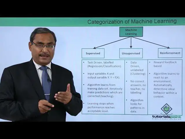
In this video we are going to discuss categorization of machine learning

Machine learning can be categorized mainly into three heads. The first one is the supervised, next one is the unsupervised, and the last one is the reinforcement

So we shall discuss one by one. Supervised learning. So supervised learning is tax-driven, labeled, and here we usually use the methods like

regression, classification, and input variables X, and if the output variable is Y, then

Y is equal to function of X. This algorithm learns from the training data set, iteratively

make predictions which are corrected and through the teaching, and learning stops when

the performance reaches to the certain acceptable level. So these are the features of supervised learning

So, it is tax driven. One tax will be given to that model after being trained and the tax is supposed to

get performed. That means the model will do some classification, that means some new data set will be given

to the model after being trained and then the model will do the classification of that given

data that is a task or some regression will be there with the help of which it can predict

some data. So, in case of continuous data, we are having this regression in case of discrete data

will be having this classification. So that is known as the tax driven

Now the question is coming, what is labeled? Why this particular data set will be called as labeled

So for this one, let us go for the next slide once

So this is our very famous Irish data set and this Irish data set we have used in our multiple

different examples in this tutorial in the implementation using Python and this particular

ID's data set here I put a part of that it is having a long data set there it is having

attributes like your sipple length sepal width pittal length and pittal width and that

is our species so this is the respective sipple length with pital length width are given

and these values are given and it is classifying it as three different types of pieces. So, that means this particular data set is having three

classes. So, one is the versicolor. This one is the setosa and the last one is the virginica

So, there are three different flowers are there and their respective four attributes are given

and the pieces has been concluded. So that is our outcome. That is our classes. So how many

classes this particular data set is having three classes? So as this outcome is also mentioned here, this outcome is mentioned

So that's why this data set will be known as the labeled data set

So that's why in the previous slide we had this one taxed event, we have discussed, and

that's why it is called labeled. So supervised learning is labeled because this very particular fact for certain attributes

the outcome is given to us. So our model will be trained with this data set and then a new data set will be given

That means the respective sepal length, sepal width, pittal length and pittal with will be given

and then our model which has been trained properly will be predicting the target flower type

That is one of the classes of this versicolor, cetosa and virginica

Let us see another example. I think that will clear about doubts

So here you see we are having muffins and cupcakes. And these muffins and cup cups we are having here

I have just put the pictures here for a better understanding. Here this is a long data set is given

What are they? They are nothing but describing the respective recipes for this muffin and cupcake

So these are the different ingredients which will be required. So flour, milk, sugar, butter, egg, baking powder, vanilla and salt

So different proportion. the respective proportions are given and then it is labeled that this particular recipe for

this cupcake this particular proportions are for this muffin so my model will get trained

and then I shall give a different proportions and then my model will tell using artificial

intelligence that this recipe is either for muffin or for cupcake so how many classes are you

having here two classes are there muffin and cupcake so in this

way this output this particular data set will be known as labeled so that means we are

having prior information and this information will be fed to the machine learning model

the model will be trained and then we shall give some some unseen input and then the

model will predict this is known as supervised learning so input variables x and output

variable y then y will be is equal to function of x

Algorithm learns from the training data set as I discussed earlier iteratively make predictions which are corrected that is the teaching So learning stops when the performance reaches to the acceptable level so now let us go for this unsupervised

learning now what is unsupervised learning it is data driven unlabelled here the method which will be using is mainly the clustering and no correct

answers no teacher no labeling algorithm looks for patterns in the data

So, here we have written the main key points of this unsupervised learning

So I think it would be better. Let us go for one example that why it is called data driven and unlabeled

Now see this particular data set for unsupervised learning. So what is happening here

You see here we're having multiple different items. Tea or coffee, sauces, confectionery, pudding, puddings and desserts, frozen, reserved blades

and so many, so many items are there. So, what are there? Actually, we are having multiple transactions, say, in a shopping mall

So, these items are there and in a particular shop rather, in these items are there

And we have considered different bills which have been made throughout, say, last 10 years

So, in the case, we are just putting 0 and 1 only to indicate that these items occurred in the same bill

And this another combination is there. only one item has been purchased frozen in another bill in this we are having

say crores of such data sets we are having crores of such records in this

data set now I shall have to find out the pattern that means which items are

occurring very commonly in one bill so here you see that is no outcome

there is not teaching there is not training there is no labelled it is data

driven so it is known as unsupervary learning. Try to get my point. Here you see that is nothing outcome. No classes are there

pre-given. So, what we are having? We are having a huge set of data. From where what we are

trying to find out? Say one particular pattern. What pattern? Which items are occurring very frequently

in the billing process? So, in the case, in the case, obviously, if we find that this item

and that item has been sold very frequently in the same bill, then you can go for some

what should I say, some offer may be given to that, some combo offer of those two items

and where to place those two items in which shelf, in which rack, where to place them

and how to place them. So, we can do the business planning and you can maintain, we can

mention the, we can implement some, some planning for that. Strategy can be also implemented

for that. So, this is known as data driven. So, data set for unsupervised learning

So, let me revise once again. This is known as unsupervised learning

That is data driven unleveled. Here we will be doing the clustering

Clustering means we are trying to find out the group of items which are having some similar

properties or which are which items are within a very small, some predefined distances within

the predefined distances. So in this way we can do the clustering

And then no correct answers, no teacher. no leveling. So this particular this particular data set will be given to our model. So

model will try to find out, we'll try to train itself and we'll try to find out some pattern

in our data. So algorithm looks for patterns in data. So that is our unsupervised learning

So let me go for the reinforcement. So that is a reward feedback based. Algorithm

learns to react on an environment automatically determine ideal behavior within a context

So, this is our reinforcement. Now, what is that actually? Let us suppose when we usually play a computer game, then most of the time, we are having

some idea. I have seen that some other person have played that game

I was with him or her. So I am having some idea. but when I'm playing with that game, so some initially I was failing to move to the next level

of the game. So what was happening? I was causing some mistakes

Some faults were there in my playing. Strategy was not good. So that's why I was missing to move to the next level

So from there I'm learning. And when I got, I got my chance to move to the next level, next level, next level, next level

each and every time I'm getting rewarded and I'm making. myself learning, I'm making myself learned that this is the way in which I should play

So, this is known as the reinforcement learning. Let us suppose when a particular kid is trying to learn how to drive a cycle, so how to do

the cycling, he or she might be having idea looking at some other people that we should

paddle, we should hold this respectively handles and so on. So, the mechanism must be known to them, but when they are learning, so they are getting

this idea, sometimes they're falling, having some painful experiences. So, from there, they're getting this idea that what has to be done, what has not to

be done sometimes the rewards are coming from the parents that you have done a good job Yes you are now a perfect rider So in those cases getting the rewards the kid is learning that how to do the cycling

So that is our reward-based reward feedback-based. Algorithm learns to react to an environment, automatically determine ideal behavior within a context

So in case of reinforcement learning, we're having two things. one is the agent and the one is the environment so agent will give some input to the

environment and environment will give some feedback to the agent and in this way the agent

will learn from the environment so this is of a machine learning so it can be categorized

into three heads supervised unsupervised and reinforcement now let us let us discuss

the machine learning coordinates so supervised learning in case of on the discrete

data will be going for classification of categorization and in case of continuous data

will be going for regression. So, in case of Irish data set whatever we discussed, then you can go for the classification

or categorization. The petrol length and simple length and width will be given to us and then a new data site

will be given to us on which we shall go for the predictions

So we can go for the classifications and here in case of predicting something where, where

we are having y is equal to function of x. So, for a new x I can calculate this value of y

So, regression can be applied in case of continuous data. In case of unsupervised learning, in case of discrete, we'll be going for clustering

Clustering I told you this one, we are trying to find out similar data in a certain

group or cluster having got either similar properties or having the distance within a certain limit

Another one is that dimensionality reduction. So question is coming in. is coming in the mind that what is the dimensionality reduction. So in statistics, machine learning

and the information theory, dimensionality reduction or dimensional dimension reduction is a process

of reducing the number of random variables under the consideration by obtaining a set of principal

variables and it can be divided into feature selection and feature extraction

So, this is our dimensionality deduction. Now, the question is coming in the mind that what is our principal variables and what

is our feature selection and feature extraction. So feature selection and feature extraction means that we know that feature selection means

we are having multiple attributes in a data set. We shall try to find out those features which is actually related with the outcome

So, we can select some of the features because if you go on dealing with huge number of features

and attributes in the data set, then obviously the computational complexity will be too high

So in that case, you can go for the feature selection and in case of feature extraction

will be going for secondary layer of some extraction from the data set

That means we are not going for the classification, but we are trying to find out some

extra information from our data set. So, let us, we shall discuss them in the later slides

So, we'll be having the clear conception. So that is known as the dimensionality reduction

So at first we're discussing with this classification and class study. So classification is the problem of identifying to which of a set of categories, also known

as classes, a new observation belongs on the basis of a training set of data containing

observations or instances whose category membership. is known to us. So, that is just considered our Irish data set, just consider our muffin

and cupcake data set. In those cases, we know the previous information because the

data set was labeled. So, now we shall try to predict on a new data, new data set given

to that. So classification is considered an instance of supervised learning and learning

where a training set of correctly identified observations are available. The corresponding unsupervised procedure is known as clustering and involves grouping data into

categories based on a measure of similarity or some distance. So we have discussed this one, that is a classification and clustering

So example, this is an example of classification problem where there are two classes

one is a low risk and another one is a high risk customers so the information about a customer

makes up the input to the classifier whose task is to assign the input to one of the two classes

after training with the past data a classification rule learned may be of the form like this

just consider this one if income is greater than theta one and savings is greater than theta two

then low risk else high risk so here we have plotted income along the x-axis

here we have plotted the savings along y axis now what is income what is the

problem actually let us suppose a credit cut company has got multiple

crores of different applications have been made by the applicants so all those application data is available now the credit cut company will decide whether they will issue a credit card for the respective applicant or not whether it is going for two classes

Low risk, credit card should be given and high risk credit card should not be allowed

So now you see when the income value is greater than theta 1 and the savings is greater

than theta 2, just look at here. So theta 1, more than theta 1, and

greater than theta 2, then that is our low risk zone. We have marked this one with some other color

Otherwise it is our high risk zone. So that is the respective clustering we have done here

So now let us go for the next one. So in this way the classification and the clustering, here we have done the classification

and whenever we are trying to find out some group of data in that case, having the similar

properties or some within a distance then we can go for the class studying in that

case. So, here we are having two classes. One is the low risk and one is the high

risk. Next one we are going for the regression. So a regression problem is when the output

variable is a real value such as dollars or say weight instead of a class. That means it is

a numeric. Estimate the relationship between a dependent variable and one or more independent

variables also known as predictors so here you can say that we are having the

sales figure for a television model can depend on several factors so that is

the screen size display type brand resolution technology etc so that will

decide the cells of that particular for the particular instrument so now this

television is having multiple different properties so this instrument we are trying to find out that what is the respective sales prediction so here

we consider just one attribute that is a screen size of the television and plot the

corresponding prices. So, here we have plotted the screen size and here we have plotted

the respective sales figure. And here we are having the screen size we have plotted and

plot the corresponding prices, that is x is equal to screen size and y is equal to sales figure

So we try to find the deletion function that best matches these two values

So here we have plotted the screen size. Here we have plotted the prices means actually you are trying to mean that one as the sales figures

So now here we are having multiple dots and we are suggesting one line that is known as

the regression line and this is the respective equation for the regression line

So for some unknown X I can find the respective Y value

So Y is equal to f of x. Next one we are going to discuss that is the dimensionality reduction

So dimensionality reduction is the process of reducing the number of random variables under consideration by obtaining a set of principal variables

So, it can be divided into feature selection and feature extraction. So, that is known as the dimensionality reduction

A data set may have hundreds of attributes, thousands of attributes. If I go on doing calculations and learning process with all those attributes, then obviously

the computational complexity will be unnecessary high. So, in those cases, we should select those attributes which are the prime attributes, also known

as the principal attributes, on which will be training our model and later we shall expect

a good prediction out of them. So this is known as the dimensionality reduction

So next we are going for the feature selection. Feature selection approaches try to find a subset of the original variables, also called the features

or attributes. It is about choosing some of the features based on some statistics

score so we might be having multiple different features so we can make those

features with some weightage values so that those features with the weightage

value smaller that means that feature is having lesser importance and those

features which are having the the weightage value higher that means that

feature is having the higher importance so in this way we can go for this

feature selection next one is the feature extraction so feature extraction transforms the data in the high dimensional space to a space of fewer dimensions, it is using

techniques, it is using techniques to extract some second layer information from the data

So, as example, you just see this one, interesting frequencies of a signal using Fourier transform

So, if we find this particular one, so you are going for a second layer of, that is a second

layer of information you are trying to find out. and that is known as feature extraction

So the data set is actually meant for something but we are trying to find out something new from that one, from that particular data set we are trying to predict something new or

calculate something new and that is known as feature extraction. Dimensionality reduction helps in data completion, reduces computational time and removes

the redundant features. So in this way we have discussed all these respective categories and different

classifications, clustering, categorization, dimensionality deductions, everything we have discussed into details. Please watch all the videos in the tutorial for your better understanding

Thanks for watching this video