Up next in 10

Understanding P-Values - A Simple Explainer
Study Note: https://biologynotesonline.com/p-value/
In this video, we delve into the concept of P-values, a fundamental aspect of statistical hypothesis testing. Designed for both beginners and those looking to refresh their knowledge, this simple explainer breaks down what P-values are, how they are calculated, and their significance in research. We will explore common misconceptions and provide practical examples to illustrate their application in real-world scenarios. By the end of this video, you will have a clearer understanding of how P-values can inform decision-making in scientific studies. Join us as we demystify this essential statistical tool! #Statistics #PValues #DataAnalysis
Website: https://biologynotesonline.com/
Facebook: https://www.facebook.com/biologynotesonline
Instagram: https://www.instagram.com/biologynotesonline/?hl=en
understanding p values in hypothesis testing,p value explained,p-value explained,understanding p-values,p-values,p-value explained in simple terms,p-values explained,p-value explained simply for data scientists,pe ratio explained simply,understanding p-value,understanding null hypothesis and p value,p-value explained in 60 seconds,significance testing explained,transistors explained,p-values in medicine,statistical significance explained,p-values defined
Show More Show Less View Video Transcript
0:00
what is a
0:01
palue a palue is the probability of
0:04
obtaining results at least as extreme as
0:06
those observed if the null hypothesis
0:08
were true to understand p values let's
0:11
visualize a normal distribution
0:13
representing test statistics under a
0:15
null hypothesis if we observe a test
0:18
statistic beyond a critical value we
0:20
enter a region of low probability under
0:22
the null hypothesis the p value
0:25
represents the probability of observing
0:27
such extreme results if the null
0:29
hypothesis were true let's clarify some
0:31
key points about p values p values
0:34
measure the strength of evidence against
0:36
the null hypothesis smaller p values
0:39
indicate stronger evidence against the
0:41
null hypothesis important to note a p
0:44
value is not the probability that the
0:46
null hypothesis is true and it is not
0:48
the probability that the results
0:50
occurred by chance now let's briefly
0:53
discuss statistical significance
0:55
typically a threshold of P less than 0.5
0:58
is used to determine significance
1:00
results with P values below this
1:02
threshold are considered statistically
1:05
significant however this doesn't
1:07
necessarily mean the effect is large or
1:09
important in a practical sense
1:11
understanding what a p value represents
1:14
is essential for correctly interpreting
1:16
statistical results
1:19
hypothesis testing provides a framework
1:22
for making decisions based on
1:25
data hypothesis testing follows a
1:27
systematic five-step process step one
1:30
state your null and alternative
1:32
hypothesis the null hypothesis
1:34
represents no effect or no difference
1:36
step two choose a significance level
1:39
known as alpha this is your threshold
1:41
for determining statistical significance
1:43
commonly set at 05 step three calculate
1:47
a test statistic from your sample data
1:49
step four determine the p value which is
1:52
the probability of observing your
1:53
results or more extreme if the null
1:56
hypothesis is true step five make a
1:59
decision by comparing the p- value to
2:00
your significance level if p is less
2:03
than alpha reject the null
2:06
hypothesis let's illustrate this process
2:08
with an example testing whether a coin
2:11
is fair step one we state our null
2:14
hypothesis that the coin is fair with
2:16
probability of heads equal to 0.5 the
2:19
alternative is that the coin is not fair
2:21
step two we choose a significance level
2:24
of 0.05 which is commonly used in
2:27
statistical testing let's say we observe
2:29
30 heads in 50 flips is this
2:31
significantly different from what we'd
2:33
expect if the coin were fair
2:38
step three we calculate the test
2:40
statistic for a binomial test our
2:42
statistic is simply the number of heads
2:44
observed under our null hypothesis of a
2:47
fair coin we would expect 25 heads in 50
2:50
flips but we observed 30 heads is this
2:53
significantly different step four
2:56
calculate the p value for a two-tailed
2:59
test we need to find the probability of
3:01
observing a result as extreme or more
3:03
extreme than 30 heads in either
3:05
direction the p value for this test is
3:07
approximately
3:09
0.103 this represents the probability of
3:12
observing 30 or more heads or 20 or
3:14
fewer heads if the coin is truly fair
3:17
step five make a decision since our p
3:20
value of 0.103 is greater than our
3:23
chosen alpha of 05 we fail to reject the
3:26
null hypothesis we conclude that there
3:28
is insufficient evidence to suggest that
3:30
the coin is unfair the observed result
3:33
of 30 heads could reasonably occur by
3:35
chance with a fair
3:38
coin the p value plays a crucial role in
3:41
hypothesis testing by quantifying the
3:44
strength of evidence against the null
3:46
hypothesis smaller p values indicate
3:48
stronger evidence against the null
3:50
hypothesis
3:52
however it's important to remember that
3:54
P values don't measure effect size or
3:56
practical significance and must always
3:59
be interpreted in the context of the
4:00
study
4:03
design now let's focus on interpreting P
4:06
values correctly p values range from 0
4:09
to 1 and serve as a universal language
4:12
for interpreting statistical test
4:13
results the most common threshold used
4:16
is
4:17
0.05 results with P values less than
4:19
0.05 05 are typically considered
4:22
statistically
4:23
significant in hypothesis testing when
4:26
the p value is less than
4:27
0.05 we typically reject the null
4:30
hypothesis indicating a statistically
4:33
significant result conversely when the p
4:35
value is greater than 05 we fail to
4:38
reject the null hypothesis suggesting
4:40
the result is not statistically
4:43
significant to visualize p values we can
4:46
look at a distribution curve the p value
4:49
represents the probability of observing
4:51
a test statistic as extreme or more
4:54
extreme than what we observed the
4:56
smaller the p value the smaller the area
4:58
in the tail of the distribution and the
5:00
stronger the evidence against the null
5:03
hypothesis at our conventional threshold
5:05
of 0.05 the critical region includes
5:08
these values in the tail larger p values
5:11
like 0.1 indicate weaker evidence
5:14
against the null hypothesis
5:16
let's look at how we can interpret
5:18
different ranges of p values p values
5:20
less than 0.001 provide very strong
5:23
evidence against the null hypothesis p
5:26
values between 0.001 and 01 offer strong
5:30
evidence values between 01 and our
5:33
typical threshold of 05 indicate
5:35
moderate evidence p values between 0.05
5:39
and 0.1 suggest weak potentially
5:41
trending evidence finally p values of
5:44
0.1 or larger generally indicate no
5:46
significant evidence against the null
5:48
hypothesis as we interpret p values it's
5:51
important to keep some key points in
5:52
mind p values do not measure the size of
5:55
an effect or tell us about practical
5:57
significance the 005 threshold is
6:00
conventional but ultimately arbitrary
6:03
what remains consistent is that smaller
6:05
p values indicate stronger evidence
6:07
against the null hypothesis
6:12
p values are frequently misunderstood in
6:14
statistical analysis let's examine three
6:17
common
6:19
misconceptions misconception number one
6:22
P values measure the probability that
6:23
the null hypothesis is true this is
6:26
incorrect the p value only tells us how
6:29
likely we would observe our data or more
6:31
extreme data if the null hypothesis were
6:33
true the correct interpretation is that
6:36
the p value is the probability of
6:38
observing our data or more extreme data
6:40
if the null hypothesis were
6:44
true misconception number two p values
6:48
indicate the size or importance of an
6:50
effect this is incorrect two studies can
6:52
have the same p value but very different
6:54
effect sizes for example these two
6:57
studies have identical p values of 0.04
7:00
04 but their effect sizes are
7:02
dramatically different the correct
7:04
understanding is that p values only
7:06
measure statistical significance not
7:09
practical significance or the importance
7:11
of
7:13
findings misconception number three p
7:16
values tell us the probability of
7:18
replicating results this is incorrect a
7:21
statistically significant result does
7:23
not guarantee the same result in future
7:25
studies the correct understanding is
7:27
that p values naturally vary from sample
7:30
to sample and a single p value cannot
7:32
predict the outcome of future
7:34
replication
7:37
attempts to summarize remember these key
7:40
points about p
7:45
values p values are just one tool in the
7:48
statistical toolbox not the final answer
7:51
to scientific questions
7:55
to calculate P values statistitians use
7:58
various methods depending on the context
8:00
and available tools common approaches
8:03
include using statistical tables
8:05
spreadsheet functions dedicated
8:07
statistical software packages or
8:09
programming languages with statistical
8:11
libraries the process of calculating p
8:14
values starts with test statistics these
8:17
statistics quantify how far our sample
8:19
results are from what we'd expect under
8:22
the null hypothesis
8:24
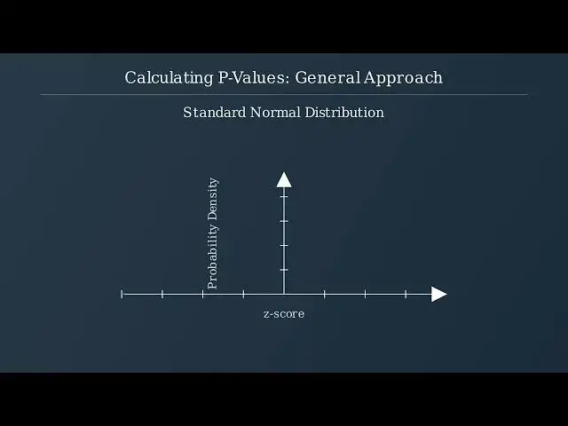
for many statistical tests p values are
8:26
calculated using probability
8:29
distributions the standard normal
8:31
distribution is commonly used for Z
8:33
tests let's look at a common example of
8:35
calculating a p value for a two-tailed Z
8:37
test if our test statistic is Z= 1.96 we
8:42
need to find the probability in both
8:43
tails beyond this
8:46
value traditionally P values were
8:49
calculated using statistical tables for
8:51
a zcore of 1.96 we would locate the
8:54
closest value in the z table we find
8:56
that for z equals 1.96 the area to the
8:59
right of this value is 0.025 for a
9:02
two-tailed test we multiply by two
9:04
resulting in a p value of
9:07
0.05 today most statistitians use
9:10
software to calculate p values
9:12
automatically spreadsheet programs like
9:14
Excel have built-in functions like
9:16
norm.s.dist to find the area under the
9:19
normal curve statistical software
9:21
packages like R SPSS or Python libraries
9:24
go even further automatically
9:26
calculating test statistics and
9:28
corresponding P values directly from
9:30
your data to summarize P values are
9:33
always derived from test statistics
9:36
while tables work for basic tests most
9:38
researchers now use software tools that
9:40
handle the calculations automatically
9:43
modern statistical tools make p value
9:46
calculations straightforward but
9:48
understanding the underlying process
9:50
helps you interpret your results
9:56
correctly to find p values for t tests
9:59
we follow a three-step process first
10:01
calculate the tstistic from your sample
10:03
data second determine the appropriate
10:06
degrees of freedom and third find the
10:08
corresponding p value using the t
10:10
distribution
10:14
the tstistic is calculated using this
10:17
formula it measures how many standard
10:19
errors the sample mean is from the
10:21
hypothesized population
10:24
mean next we determine the degrees of
10:27
freedom for a one sample t test the
10:29
degrees of freedom equals sample size
10:31
minus one for a two sample t test it's
10:34
the sum of both sample sizes minus two
10:37
degrees of freedom represent the number
10:39
of independent values that can vary in
10:41
the
10:44
calculation finally we use the t
10:46
distribution to find the p value that
10:49
corresponds to our calculated tstistic
10:51
and degrees of
10:53
freedom let's work through a practical
10:56
example imagine we're testing if a new
10:59
study method improves test scores we
11:01
have a sample of 16 students with a mean
11:04
score of 78.5 and a standard deviation
11:07
of 8.1 we want to test if this is
11:10
significantly higher than the previous
11:12
average of
11:14
75 let's calculate the t statistic using
11:17
our formula we substitute our values
11:20
sample mean 78.5 hypothesized mean 75.0
11:24
standard deviation 8.1 and sample size
11:27
16 we simplify step by step the
11:29
square of 16 is 4 dividing 8.1 by 4
11:32
gives us 2.025 finally dividing 3.5 by
11:36
2.025 gives us a tstistic of 1.728 the
11:40
degrees of freedom equals sample size
11:42
minus 1 which is
11:45
15 now let's find the p value using the
11:48
t distribution with 15 degrees of
11:50
freedom our tstistic is
11:52
1.728 for a one-tailed test we're
11:55
interested in the probability of
11:57
observing a t value this extreme or more
11:59
extreme in the direction of our
12:01
alternative
12:04
hypothesis let's compare one-tailed and
12:06
two-tailed tests using our example in a
12:09
one- tailed test we're only concerned
12:11
with the probability in one direction in
12:13
our example the p value is approximately
12:16
0.052 for a two-tailed test we consider
12:19
both directions the p value is
12:21
approximately 0.104 104 which is twice
12:24
the one tailed p
12:27
value let's make a decision based on our
12:30
p values and our chosen significance
12:32
level of 0.05 for our one-tailed test
12:35
the p value is greater than alpha so we
12:38
fail to reject the null hypothesis this
12:40
means there is insufficient evidence
12:42
that the new study method significantly
12:45
improves test scores at the
12:47
0.05 significance level
12:54
kaiquare tests are used to analyze
12:56
categorical data and determine if
12:58
there's a significant relationship
13:00
between
13:01
variables the kiquare statistic compares
13:04
observed values to expected values using
13:07
this
13:08
formula let's work through an example of
13:10
a kiquare test of independence to see if
13:13
music preference is related to age group
13:16
here's our observed data in a
13:17
contingency table we have three age
13:19
groups and four music genres with the
13:22
number of people in each
13:24
category first we need to calculate the
13:27
expected values for each cell in our
13:29
table we multiply the row total by the
13:32
column total then divide by the grand
13:35
total next we calculate the kaiquare
13:38
statistic by summing the squared
13:39
differences between observed and
13:41
expected values divided by the expected
13:44
values
13:46
we calculate the degrees of freedom by
13:47
multiplying rows minus 1 by columns
13:49
minus 1 in our example that's 2 * 3
13:53
giving us degrees of
13:56
freedom finally we use a k square
13:58
distribution table or calculator to find
14:00
the p value with a k square statistic of
14:04
26.14 and 6° of freedom we get a p value
14:07
less than 0.1 since our p value is less
14:11
than 05 we reject the null hypothesis we
14:14
conclude that there is a significant
14:16
relationship between age group and music
14:20
preference to summarize kaiquare tests
14:23
analyze relationships between
14:25
categorical
14:26
variables we calculate expected values
14:29
find the kaiquare statistic determine
14:31
degrees of freedom and interpret the p
14:33
value to draw conclusions about our
14:36
data in scientific research p values
14:40
have become a critical gateway for
14:41
publication many journals and fields
14:44
traditionally require results to meet
14:46
the P less than .005 threshold to be
14:49
considered publishable this has led to a
14:52
binary classification system where
14:54
results are simply categorized as either
14:56
statistically significant or not
14:59
significant an important distinction
15:01
exists between statistical significance
15:03
and practical
15:05
significance statistical significance
15:07
indicated by a p value below 05 simply
15:11
tells us that we can detect an effect
15:13
practical significance however addresses
15:15
whether the effect is large enough to
15:17
matter in real world
15:19
applications with large enough sample
15:21
sizes even tiny inconsequential effects
15:24
can achieve statistical
15:27
significance the scientific community
15:29
has been grappling with what's known as
15:30
the replication crisis studies have
15:33
shown that many published findings with
15:36
significant p values fail to replicate
15:38
in subsequent
15:39
research one contributor to this problem
15:42
is p hacking where researchers
15:44
manipulate their analysis methods until
15:46
they achieve a p value below
15:48
0.05 publication bias also plays a role
15:52
as journals tend to publish only studies
15:54
with statistically significant results
15:56
creating a skewed scientific record
16:00
let's examine how P values are typically
16:02
reported in scientific papers research
16:05
papers typically report the p value
16:07
alongside the test statistic sample size
16:09
and degrees of freedom increasingly
16:12
journals require reporting effect sizes
16:15
and confidence intervals to provide a
16:17
more complete picture of the
16:19
results when interpreting research
16:21
findings p values should never be
16:24
considered in isolation a more complete
16:26
picture emerges when p values are
16:28
interpreted alongside effect sizes
16:31
confidence intervals and within the
16:32
context of prior research pre-registered
16:35
studies where methods and analyses are
16:37
specified before data collection help
16:39
prevent packing and increase
16:42
credibility and finally successful
16:44
replications of findings provide the
16:46
strongest evidence for genuine effects a
16:49
thorough evaluation of research requires
16:51
considering the interconnection between
16:53
statistical significance effect size and
16:56
the broader research
17:00
context modern approaches and
17:02
alternatives to p values have emerged in
17:04
response to their limitations and misuse
17:07
in 2016 the American Statistical
17:10
Association issued a statement
17:12
addressing the proper use and
17:13
interpretation of P values the statement
17:16
emphasized that P values don't measure
17:18
effect size or importance and scientific
17:21
conclusions shouldn't be based solely on
17:23
P values it noted that P values can be
17:26
influenced by sample size not just
17:28
effect and proper inference requires
17:30
transparency and full
17:33
context let's explore alternatives and
17:36
complimentary approaches to P values
17:38
that can provide more nuanced
17:40
information confidence intervals provide
17:42
a range of plausible values for the
17:44
parameter of interest unlike P values
17:47
they show both precision through the
17:49
width of the interval and magnitude
17:51
through its location a 95% confidence
17:54
interval contains the true parameter
17:56
value in 95% of repeated
17:59
samples effect sizes provide a
18:02
standardized measure of the magnitude of
18:03
an effect common measures include Coen's
18:06
D odds ratios risk differences and
18:09
correlation coefficients unlike P values
18:12
effect sizes are independent of sample
18:14
size and facilitate comparison across
18:17
studies beijian methods incorporate
18:20
prior knowledge with new evidence to
18:22
produce posterior probability
18:23
distributions for parameters unlike
18:26
frequentist approaches Beijian
18:28
statistics allows for direct probability
18:30
statements about hypotheses and
18:32
naturally updates beliefs as new data
18:36
emerges multiple comparison corrections
18:39
address the inflation of type one error
18:41
when conducting many statistical tests
18:44
simultaneously methods like boneroni
18:46
control the family-wise error rate by
18:48
dividing alpha by the number of tests
18:51
less stringent approaches like the false
18:53
discovery rate control the proportion of
18:55
false positives among rejected null
18:59
hypothesis let's explore best practices
19:02
for responsible statistical analysis in
19:04
the modern era report effect sizes
19:07
alongside P values to communicate
19:10
practical
19:11
significance provide confidence
19:12
intervals for parameter estimates to
19:14
show precision and magnitude consider
19:17
basian alternatives when incorporating
19:19
prior knowledge is valuable pre-register
19:21
analyses to avoid P hacking and
19:23
selective reporting account for multiple
19:26
comparisons when conducting numerous
19:28
tests and report exact p values rather
19:32
than simply stating significance
19:33
thresholds in conclusion p values remain
19:36
a valuable statistical tool when used
19:39
appropriately and complemented with
19:41
other approaches by combining p values
19:44
with effect sizes confidence intervals
19:46
and other methods researchers can
19:48
provide a more complete and nuanced
19:50
statistical story that advances
19:52
scientific understanding
#Statistics